Exercise: Stable Zone Unmixing
Stable Zone Unmixing will compare pairs of classes to determine a subset of wavelengths that maximizes spectral separability between the classes, while minimizing within class variability (Somers et al., 2010). In principle, this should produce increased fraction accuracy, while decreasing run times because fewer wavelengths are being used.
Spectral Weighting (the other option), should, in principle, generate a similar result, but is likely to be significantly slower because it retains all wavelengths in the mixing process, while adding the calculations of weighting factors, so it is likely to be even slower than the original three endmember model.
Data used
- demo2.sub: a subset from the 2011 image from Goleta, Santa Barbara.
- roberts_et_al_2017_final.sli
Exercise
We will run this unmixing twice, once with and once without Stable Zone Unmixing, in order to be able to compare the result:
Spectral Library:
- Select the library roberts_et_al_2017_final.sli
- Select the metadata class named Level_2.
- The algorithm automatically selects all 2- and 3-EM models.
Constraints:
We will accept physically reasonable fractions (min=0, max=1.0), physically reasonable shade (min=0,max=0.80) and set the RMSE constraint to 0.025.
Input image:
- Select the image demo2.sub.
Advanced MESMA Algorithms:
- The second time toggle on Use band selection. You can leave the default correlation values as they are.
Run MESMA:
- We can change the output name to demo2_szu and make sure the output opens in QGIS.
- Click OK.
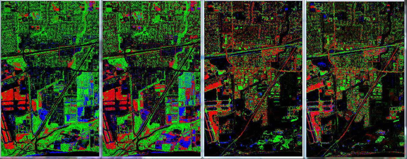
Examine your model output as we did before, loading a false color composite, NPV-GV-Soil fraction image, Paved-Roof-Rock fraction image and RMSE.
Comparing this to the original model run, we see they are qualitatively very similar. In a few areas in the southeast, the RMS appears slightly higher in this version. However, we also see that soils mapping has improved, with soil fractions now modeled in areas we know to be soil, in some areas previously mapped as roof. SZU tends to favor higher complexity models, whereas using all wavelengths tends to favor simpler models. Improved performance for mapping soils is much more evident by direct comparison.
The image below shows the original model on the left and the SZU model on the right for NPV-GV-Soil and Paved-Roof-Rock. An arrow marks one area where the models differ significantly.
The SZU version modeled all but 7k pixels, taking under 2 minutes. The original model had more un-modeled pixels (10k) and took over 8 minutes. At this stage, we do not know which model is more accurate, although we would suggest that the SZU version may be slightly more accurate. However, the SZU version is significantly faster. Assuming the factor of seven in run time improvement is consistent, our four-endmember model would have taken 31 minutes instead of 278.
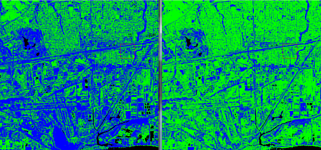
We can also verify that SZU selects for higher complexity by comparison to the original model using all wavelengths. The figure on the left shows that the original model modeled most of the image with two endmember models (blue), whereas the SZU version tended to favor three endmember models.
For issues, bugs, proposals or remarks, visit the issue tracker.