Exercise: MESMA in QGIS

For issues, bugs, proposals or remarks, visit the issue tracker.

While many algorithms can classify images, MESMA’s strength is in modeling mixtures of endmembers across multiple levels of complexity, ranging from simple mixtures of a single endmember and shade (two endmember model) to more complex mixtures requiring a total of three or four endmembers. When used for more complex mixing models, the fractions for each endmember within selected models become a valuable output from MESMA.

However, the trade off of more complex models is a much larger number of potential models being compared, which lengthens run times.

The procedure we often use is to start with a two-endmember model to classify the image, than prune that model to produce a better performing subset. This subset can be then used as a library for a three, four or five endmember model.

However, keep in mind several important facts:

• A library that works well for two-endmember classification may include some endmembers that are mixtures.
• Some classes which are suitable for a two-endmember classification may not be suitable at higher levels of complexity. Two good examples in this tutorial include water, which will be mapped in many lower reflectance areas, and artificial turf, which is a pretty rare class and probably does not form many three or more endmember mixtures.
• Large libraries can generate a very large number of models. For example, a library with 10 models in each of 6 classes will generate 60 2-EM, 1500 3-EM and 20000 4-EM models! Reducing the number of endmembers and/or the number of classes will reduce run times.
• Many spectra which may represent a viable class at one level may be spectrally degenerate at a higher level of complexity and thus have little actual impact on the fractions. A model becomes spectrally degenerate when it can be unmodeled as a combination of two other endmembers or is spectrally similar enough to another endmember it has little impact on the fractions.

We will start with a classification, using MESMA to classify the images based on two endmember models. We will evaluate model performance using the metadata files and remove any poorly performing models. Then we will follow with a three and four endmember model where we will only examine fraction performance.

Data used

We will unmix two images:

• 010614r4_4-5_clip: an AVIRIS scene from 1998, used for simple SMA with no fraction constraints.
• demo1.sub: a subset from the 2011 image from downtown Santa Barbara.

We will use the libraries that were created in the CRES, EMC and IES exercises:

• 010627_westusa_cres.sli
• roberts2017_urban_emc_opt.sli
• roberts2017_urban_ies.sli
• roberts_et_al_2017_final.sli

Simple SMA with no fraction constraints

To run Simple SMA, you can run as many endmembers as is reasonable given the dimensionality of the data, although four is typical.

Most often users will model GV, NPV, Soil and Shade for vegetated landscapes. For urban landscapes, an impervious surface endmember is often used. You are free to experiment with other endmember combinations (say muddy water vs clean water or impervious vs soil, or ash vs soil).

In most simple SMA cases, we prefer to run models with only one constraint on the fractions, namely that they sum to 1. Negative or super positive fractions are allowed.

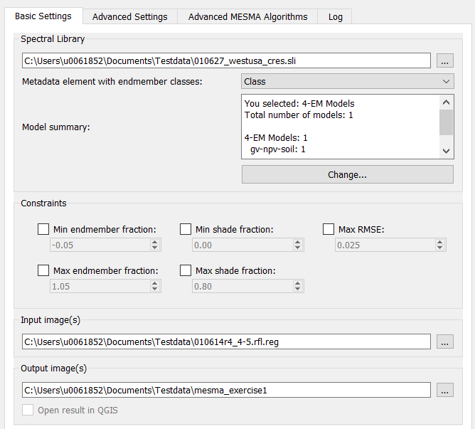
Spectral Library:

• Select the library 010627_westusa_cres.sli.
• Select the metadata class named Class.
• The algorithm automatically selects all 2- and 3-EM models. We change this to use only the 4-EM complexity level. This results in 1 model.
• Check on the Advanced Settings tab that the Reflectance scale factor is automatically set to 1000.

Constraints:

• We don’t set any constraints.

Input image:

• Select the image 010614r4_4-5_clip

Run MESMA:

• We can change the output name to mesma_exercise1 and make sure the output opens in QGIS.
• Click OK.

Expect it to take a few minutes. Don’t be alarmed if QGIS freezes for the duration of the calculations.

The output RMSE can be found in the image named _rmse and the fractions are in the image named _fractions.

You will note that the fraction image looks good, but has a fairly large number of super positive and negative fractions. The NPV and GV fractions are most reasonable in senescent grasslands and chamise, but tend towards low to negative NPV in riparian areas, and oak forests (Clearly a limitation of CCEOLSTCK). Golf courses are particularly bad.

The RMSE is generally low (often less than 1%), but highest in urban areas (often over 2.5%). Given that our best model selections were for chamise, grassland and soils, these results are not unexpected. To better model oaks, we would need a better reference endmember than the ones we had in the reference library.

Running MESMA as a classifier with a two-endmember model

MESMA can be used as a classification algorithm, by picking the two endmember model (one endmember + shade) that fits each pixel spectrum with the lowest RMSE. Run in this way, MESMA can account for variations in the brightness of pixel spectra, but not mixing between multiple material types unless endmembers representing those mixtures are included in the endmember library.

In addition to the fractions of the non-shade and shade endmembers, MESMA will output the class of the best fit non-shade endmember to provide a classified image.

Spectral Library:

• Select the library roberts2017_urban_emc_opt.sli (this is the library we created with EMC).
• Select the metadata class named Level_2. This will give us eight classes: gv, npv, soil, rock, roof, paved and water.
• The algorithm automatically selects all 2- and 3-EM models. We change this to use only the 2-EM complexity level. This results in around 150 models.

Constraints:

We will accept physically reasonable fractions (min=0, max=1.0), physically reasonable shade (min=0,max=0.80) and set the RMSE constraint to 0.025.

Input image:

• Select the image demo1.sub.

Run MESMA:

• We can change the output name to mesma_exercise2 and make sure the output opens in QGIS.
• Click OK.

Expect it to take a few minutes. Don’t be alarmed if QGIS freezes for the duration of the calculations.

Remove under-performing models

A two-endmember model, generated using a model pruned either using EMC, IES or some combination, is not necessarily the ideal model. First and foremost, the utility of the model depends on how representative the library is of the image. If the library is very good, minimal pruning may be necessary.

However, if the pruning technique has either selected models that are extremely rare in the image, or models that tend to be confused with materials outside of their class, the classes will either be under-mapped or over-mapped. Either case is a problem, but we also have the tools on hand to address both.

The first approach is to cull out under-performing models. For this, we will use the MESMA Models Viewer.

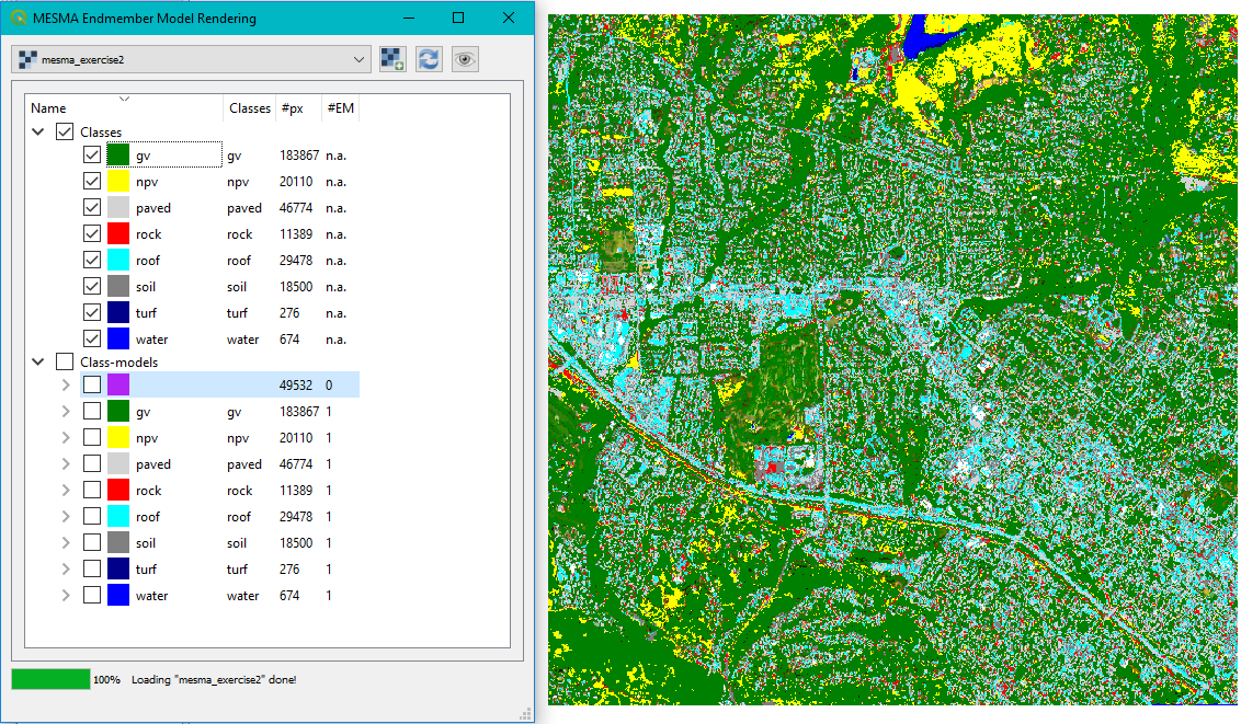
A small portion of the image (a little under 50k pixels) remained unclassified. By sorting the models on number of pixels, we can easily find several under-performing models.

As an exercise, you can find all poorly performing models (for this exercise let’s say 20 or less pixels). You’ll find around 30 models. Simultaneously open the spectral library to analyze the models.

Some poorly performing models include:

• GV: MIRRA STAR_JASMINE
• PAVED: TILE_ROAD ASPHALT_ROAD CONCRETE_ROAD
• ROOF: ASPHALT_ROOF WOOD_SHINGLE_ROOF TILE_ROOF
• NPV: WOOD NPV (LITTER)
• SOIL: ASPHALT_GRAVEL

Some caution should be used in discarding a model, in case it is appropriate for another image.

Remove models that are modeling incorrect classes

The previous exercise works well for discarding models that do not model much area. However, it does not tell us anything about models that are modeling a large area of the wrong material.

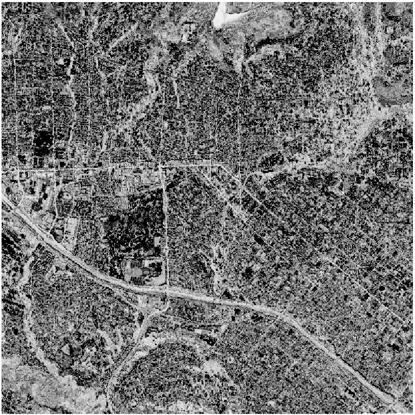
This has to be done by also examining the RMSE and fraction images:

• load one image for the RMSE
• load one image for each fraction band
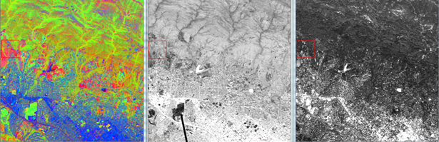
• load the original image as RGB or false color composite (1650 nm, 830 nm, and 650 nm as R, G, and B)

The image below shows from left to right, examples of the RMSE, GV, NPV and Paved fractions (using single band gray).

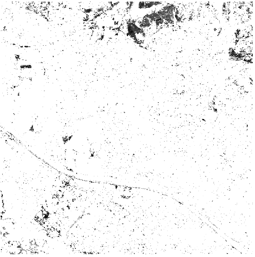
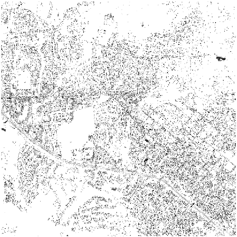
Examining the image, we see that qualitatively, the fractions look good. Areas of obvious GV are mapped as GV, the same goes for NPV and soil. Roofs, paved areas and rock as a group are mapped correctly, but seem to be mixed a lot.

Try to identify the most problematic rock spectrum. First visualize all rock models and visualize them one by one. RDP_117_X2486_Y202 seems to be map a lot of highway.

You can do this for all data types. Obviously, this kind if pruning is only possible with an in-depth knowledge of the study area.

Following is our own assessment of bad models: - BAPI05_X344_Y234 - CISP_09_X632_Y378: tends to model many urban trees and shrubs - EUSP_I04_X290_Y243: over maps Eucalyptus - MARSH01_X405_Y302 - BRNI_I02_X695_Y802: possibly okay, certainly not safe to discard - concrete_bridge_1_X2667_Y700: tough call, mapping paved surfaces, but not concrete bridges - tennis_court_n1_X1321_Y399: mapping roads

Using the IES library

Do the exact same exercise with the IES library at Level 2 and display the results. You can also display the fraction images as RGB images, using three different fractions for R, G and B, e.g. NPV-GV-Soil and Paved-Roof-Rock, like in the images below:

We see another model that looks, qualitatively, to be quite good. Areas of green vegetation are modeled with high GV fraction and senescent grassland is mapped in the north. Paved looks quite good with roads mapped in red. Roof looks generally good, but at least one area is probably soil mapped as roof.

We will use a combination of the MESMA Model Viewer and the Spectral Library to evaluate model performance, as we dit before. Right away we find quite some under-performing models (around 60), especially with roof an paved spectra.

To find over-mapping models, carefully compare the false color composite to the NPV-GV-Soil image to find areas that clearly look to be mapped wrong.

Generating the final libraries

Having identified poorly performing models with the EMC and IES libraries, you can now remove them using the spectral libraries tool.

Running MESMA for a three endmember model

Spectral Library:

• Select the library roberts_et_al_2017_final.sli, which has much of its spectral degeneracy removed
• Select the metadata class named Level_2.
• The algorithm automatically selects all 2- and 3-EM models.

Constraints:

We will accept physically reasonable fractions (min=0, max=1.0), physically reasonable shade (min=0,max=0.80) and set the RMSE constraint to 0.025.

Input image:

• Select the image demo1.sub.

Run MESMA:

• We can change the output name to mesma_exercise4 and make sure the output opens in QGIS.
• Click OK.

Expect it to take a few minutes. Don’t be alarmed if QGIS freezes for the duration of the calculations.

A high proportion of the image was modeled, with only 1695 pixels un-modeled. Much of the un-modeled area is water. Examine the models by displaying a false color composite, NPV-GV-Soil fractions, Paved-Roof-Rock fractions and the RMSE.

The images below show the RMSE and the NPV-GV-Soil fractions images:

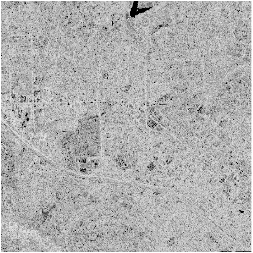
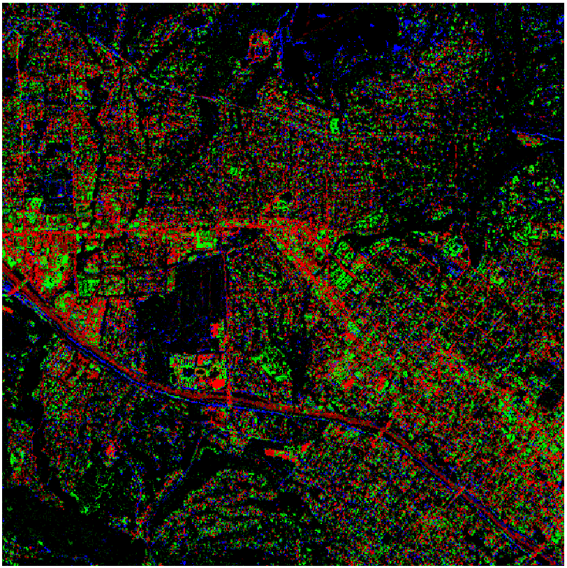
Overall, this as a very satisfactory model. Looking at the RMS error image, we see a few areas of high RMS, one of which some miss-mapping between paved an roof. This suggests to that we are short a critical endmember. Water is also an area of high error, which is normal, as water was taken out of the model.

Running MESMA for a four endmember model

Spectral Library:

• Select the library roberts_et_al_2017_final.sli
• Select the metadata class named Level_2.
• The algorithm automatically selects all 2- and 3-EM models. Also select 4-EM models. MESMA warns us that we will run 53 637 models. Depending on your RAM and processors, this will likely take more than two hours.

Constraints:

We will accept physically reasonable fractions (min=0, max=1.0), physically reasonable shade (min=0,max=0.80) and set the RMSE constraint to 0.025.

Input image:

• Select the image demo1.sub.

Run MESMA:

• We can change the output name to mesma_exercise5 and make sure the output opens in QGIS.
• Click OK.

Load a false color composite, NPV-GV-Soil Paved-Roof-Soil and RMS images. Qualitatively this image looks quite good. Unlike the EMC version, soils appear to be well mapped and the RMSE is substantially lower throughout. This is a good model.

Looking at the metadata, we see that this model captured all but 7,900 pixels, leaving only 2.2% of the image unmodeled (and this is mostly water). There are no substantial fraction errors that are evident.

Grasslands are often modeled with two endmembers, orchards with three endmembers, and the urban areas often require four endmember models.