QGIS GUI

Select the spectral library.
The reflectance scale factor is automatically detected as 1, 1000 or 10000, but can be changed in the advanced settings.
Note
Reflectance data can be saved to file as reflectance values (i.e. values between 0 and 1) or the data can be multiplied by a scale factor (usually by 1000 or 10000). This is done to be able to store the data as integer values (no comma’s), because integers require less memory. Although this is more efficient storage-wise, it has as a result we have to divide the data values again before processing.
The software tries to auto detect this scale factor, but does not always succeed (in the case of masked data with a lot of zero’s along the edges, or in the case where the scale factor is a different number, like 256). Double check this value in the Advances Settings tab.
Select the metadata element that divides the spectra in the library into classes.
The tool automatically selects all 2 and 3-EM models for you. To change the selected models, click Change…
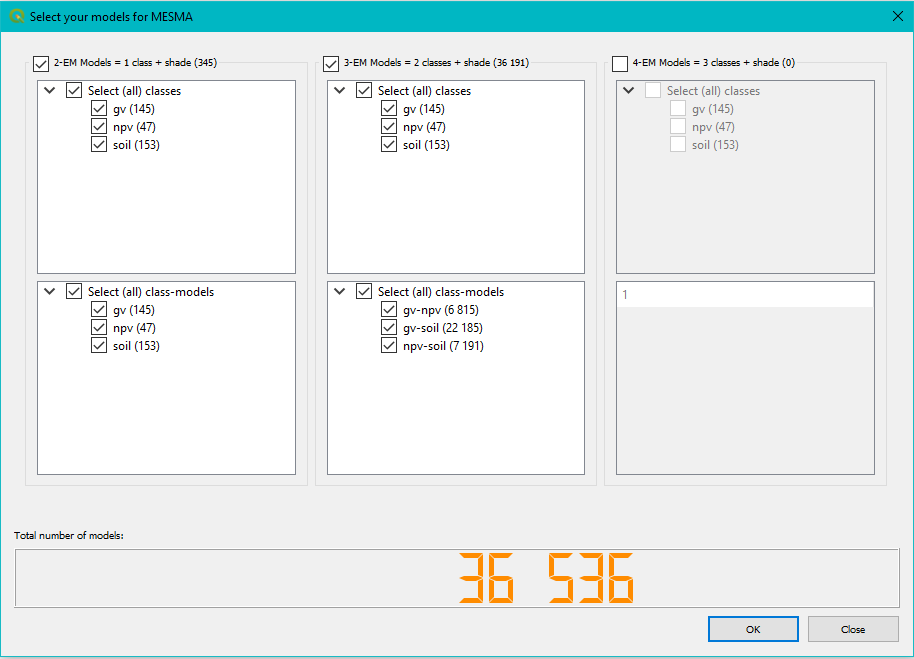
Choose the model complexity (2-EM Models, 3-EM Models, …). For a classification exercise, a user would select a 2-EM Models (endmember + shade).
Note
The user can select as many complexity models as there are classes. However, be warned, the fundamental dimensionality of a pixel is usually no higher than four, and at times five, so selecting a nine endmember model would require considerable computation that most likely will reduce accuracy.
Within a complexity level, select which classes and class-models you would like to use.
The number at the bottom indicates the total number of models and warns the user if numbers get out of hand (green is good, red is bad). Mind though that this can vary with computer power and is mere an indication.
Go to the Advanced Settings if you want to change the Multi-level Fusion Threshold. This is the threshold that determines how much the RMSE must improve between model complexity levels, before the more complex model is selected. This defaults to 0.007 following multiple papers (e.g. [Roberts2012]).
The Advanced Settings also allow the user to include non-photometric shade.
Set the constraints (optional, but by default on):
- Minimum endmember fraction: the lowest allowable fraction value. Cannot go below -0.5. Default -0.05.
- Maximum endmember fraction: the highest allowable fraction value. Cannot go over 1.5. Default 1.05.
- Minimum shade fraction: the lowest allowable shade fraction value. Setting the minimum will prevent negative shade fractions and can better discriminate endmembers by brightness. Default 0.
- Maximum shade fraction: the highest allowable fraction value. Setting this can help to ensure that water and deep shadows remain un-modeled. Default 80%. However, recently Wetherley et al. [Wetherley2018] have demonstrated that a lower setting (20%) better discriminates between turf grass and trees.
- RMSE constraint: the maximum allowable model RMSE.
- In the Advanced Settings, it is also possible to set the Residual Constraint. It is composed of two components: a constraint threshold and a number of consecutive bands upon which to apply the constraint. Selecting a threshold of 0.025 and a count of 7, for example would exclude all models which produce residual spectra that exceed 0.025 for 7 consecutive bands. By default this option is not used, and in practice models with high RMSE also fail a residual constraint.
Note
Pixels that do not meet these constraints are classified as ‘unmodelled’ in the output.
Select the image or images that will be unmixed.
- The reflectance scale factor is automatically detected as 1, 1000 or 10000, but can be changed in the advanced settings.
An output image name is automatically generated but can be changed when only one image is selected.
- The default output name is InputImageName_mesma_YYYYMMDDThhmmss.
- The Advanced Settings also allow the user to create a Residual Image. By default option is off as residuals images are large files and therefore require extra storage and incur computational costs to write them to file. Residual images contain the model residual spectra stored in floating point data type. For each pixel the residual spectrum is calculated as the image spectrum minus the model spectrum, where the model is the best fit model for that pixel as determined by minimum RMSE. Because the residuals image has the same number of bands as the input image and is a floating point image it is as large or larger than the input image.
Advanced MESMA algorithms are available in the last tab:
- In Spectral Weighing (slow) [Somers2009], all bands are used, but a weighing factor is used to reduce the influence of bands that do not improve endmember separability.
- Band Selection employs Stable Zone Unmixing (SZU) [Somers2010] and generates a reduced band set, where only those bands that best discriminate endmember pairs are retained.
Additional options:
- The Save Settings button allows the user to save all selected settings to a text file. This option is included to capture complicated settings which are time-consuming to input and prone to errors when reproducing.
- The Reload Settings button allows the user to reload the exact same model parameters at a later date to either modify them or to apply them to a different image.
Processing notes:
Note that if large images and/or a large number of models are used, this may require a long time to complete.
The use of a default naming convention based on time and date is very convenient. However, when running many models, it can result in a plethora of output files that differ only in the timing of the run. If you generate a product you like very much, and what to find it again easily, you might consider renaming
Issue Tracker:
For issues, bugs, proposals or remarks, visit the issue tracker.
CITATIONS
| [Roberts2012] | Roberts DA, Quattrochi DA, Hulley GC, Hook SJ and Green RO. 2012. Synergies between VSWIR and TIR data for the urban environment: An evaluation of the potential for the Hyperspectral Infrared Imager (HyspIRI) Decadal Survey mission. Remote Sensing of Environment, volume 117, p. 83-101. |
| [Somers2009] | Somers B, Delalieux S, Stuckens J, Verstraeten WW and Coppin P. 2009. A weighted linear spectral mixture analysis approach to address endmember variability in agricultural production systems. International Journal of Remote Sensing, volume 30, p. 139-147. |
| [Somers2010] | Somers B, Delalieux S, Verstraeten WW, van Aardt JA, Albrigo L and Coppin P. 2010. An automated waveband selection technique for optimized hyperspectral mixture analysis. International Journal of Remote Sensing, volume 31, p. 5549-5568. |
| [Wetherley2018] | Wetherley EB, McFadden JP and Roberts DA. 2018. Megacity-scale analysis of urban vegetation temperatures. Remote Sensing of Environment, volume 213, p. 18-33. |